Cortical GABAergic cell types from clusters of MERFISH markers for the detection of cortical CEFv3

Note that the precision of this analysis is highly dependent on the accuracy of CCFv3 registration. There might be incorrect registration in the adjoining CCFv3 regions, something we are working to improve.

Cell signatures from different regions are found in each region of the CEFv3 and confusion is usually only found in neighboring regions. One exception is cortical GABAergic cell types, which are shared across all cortical areas as we previously reported23,26 (Extended Data Fig. 16b). We could still observe partial separation of upper and lower cortical layers due to enrichment of CGE and MGE neurons respectively. There are only a few subclasses that colocalize with other subclasses in the same group, except for a couple of them that are highly Heterogenous.

The class, subclass, supertype and cluster were organized into a hierarchy which made the complexity easy to comprehend at each level. We first defined subclasses by clustering the clusters. This was performed by Jaccard–Leiden clustering using the average expression of 534 transcription factor marker genes of all the cells in each cluster, using 5 KNNs, and varying the resolution index of Leiden algorithm at 0.1, 0.2, 1, 5 and 8. We tried clustering using either all 8,460 marker genes or 534 transcription factor marker genes only, and found the result based on transcription factors recapitulate existing knowledge of cell types including spatial distribution and lineage relationships better. 48 groups were created at resolution index 0.2, and another 240 groups were created at resolution index 8.

To make comparisons between cells from different platforms, we projected gene expression from the 10xv2 to the 10xv3 dataset. The basic idea is to compute the KNNs (k = 15 by default) among the reference cells for each query cell and use the average expression of these neighbours for each gene as the imputed values. One of the decisions that needs to be made is how far the distance metric should be. We chose cosine metric due to overall conservation of gene expression at the cluster level (Extended Data Fig. 7d). The inference is not perfect and using too many genes could make it more susceptible to platform differences. Therefore, we used the 500 MERFISH marker genes to compute KNNs, since they provide good predictive powers at all levels of the hierarchy and show high correlation at the cluster level between 10xv2 and 10xv3 platforms (median 0.945, Extended Data Fig. 7d). A good starting point is the imputation accuracy for separating fine cell types, but it could be improved further by incorporating cluster-level DEGs, as fewer are included in the 500 MERFISH gene list. To solve this problem, we leveraged the established cell-type hierarchy and performed imputation iteratively, first at top level and then within each class and subclass. At the top level, we used the 500 MERFISH genes to compute KNNs and then imputed the expression of all 8,460 marker genes. For each subsequent iteration, we only computed the KNNs among the reference cells within the same class/subclass as the query cells using the top 10 DEGs between clusters within the given class/subclass; we then updated the imputed expression of the top 20 DEGs between clusters within the given class/subclass.

We used CCFv3 (RRID: SCR_002978) ontology22 (http://atlas.brain-map.org/, Supplementary Table 1) to define brain regions for profiling and boundaries for dissection. We used sampling at top-ontology level to make sure all the parts of the brain are covered. 1d,e and Supplementary Table 3). Microdissections of small regions were difficult to navigate. Therefore, joint dissection of neighbouring regions was sometimes necessary to obtain sufficient numbers of cells for profiling. The data from the CCFv3-based microdissections showed that they were most accurate at the cell subclass and brain region levels.

We found out after registration that there were only 7 small subregions completely missed in the MERFISH dataset for frontal pole, layer 1 and accessory olfactory bulb.

The Allen CCFv3 was aligned by matching the scRNA-sq derived region labels to their corresponding parcellation. Each region’s label map was created by converting the assigned cells in a 1010 m grid to the initial configuration using rigid transforms. Using the corresponding anatomical labels, the ANTS registration framework was used to establish a 2.5D deformable spatial mapping between the MERFISH data and the CCFv3 via three major steps: (1) A 3D global affine (12 dof) mapping was performed to align the CCFv3 into the MERFISH space. This generated resampled sections from the CCFv3 that provided section-wise 2D target space for each of the MERFISH sections. Since the CCFv3 is a continuous label set with isotropic voxels, this avoids interpolation artifacts that can result if resampling is performed on the MERFISH data instead, which has large section gaps, and can contain missing sections. Each MERFISH section was aligned to match the global nature of the CCFv3 brain after a resampled section was established. This addressed different alignments from the initial manual stacking and provided a global mapping for the local mappings. (3) Finally, a 2D multi-scale, symmetric diffeomorphic registration (step size = 0.2, sigma = 3) was used on each section to map local anatomic differences between the corresponding MERFISH and CCFv3 structures in each section. It is possible to point-to-point map between the original MERFISH coordinate space and the CCFv3 space from preserved and concatenated Global and section wise mappings from each of the registration steps.

For staining the tissue with MERFISH probes a modified version of instructions provided by the manufacturer was used. The manufacturer provided instructions on how the solutions were to be prepared. For hybridization samples were removed from the 70% ethanol and washed in a petri dish containing VIZGEN sample prep buffer (VIZGEN, 20300001). Sample prep buffer was aspirated, and the samples were equilibrated with 5 ml of VIZGEN formamide wash buffer (VIZGEN, 20300002) in a humidified incubator at 37 °C for 30 min. Formamide wash buffer was removed via aspiration and a 50-μl droplet of MERSCOPE Gene Panel Mix was added onto the centre of the tissue section. Next, the tissue section was covered with parafilm and stored in a humidified 37 °C cell culture incubator for 36–48 h.

The sections were prepared for gel to fully polymerize by keeping them at room temperature for 1.5 hours. The section should be incubated in 5 ml of VIZGEN Clearing Solution for at least 24 h before being placed in a humidified oven to get rid of the tissue.

Mice were anaesthetized with 2.5–3% isoflurane and transcardially perfused with cold, pH 7.4 HEPES buffer containing 110 mM NaCl, 10 mM HEPES, 25 mM glucose, 75 mM sucrose, 7.5 mM MgCl2, and 2.5 mM KCl to remove blood from brain123. The brain was frozen for 2 minutes and moved to 80 C, where it would stay for a long time after a freezing protocol was developed.

Integrated UMAP: A High-Resolution Atlas of Cell Types in the Whole Mouse Brain Using Taxonomy Tree and Clustering Methods

The mechanism for co-transmission of dopamine and GABA in theSTR is unconventional, since it does not depend on the creation of cell-based habituated dopaminergic cells but on pre-synaptic absorption from the extracellular space by the S LC6a1 (GAB1). However, because Slc6a1 is widely expressed in all GABAergic neurons, as well as astrocytes, and even many subcortical glutamatergic neurons, it is unclear to us how widely applicable this unconventional mechanism (which bypasses all GABA-synthesizing enzymes) is. We didn’t include Slc6a1 because we wanted to minimize false positives, even at the risk of having some false negatives.

We first annotated each subclass with its most representative anatomical region(s) and named the subclass using the combination of its representative region(s), major neurotransmitter, and in some cases one or two marker genes. In order to assign subclass IDs to the subclasses, we ordered them based on the taxonomy tree. Supertypes were defined by combining the subclass name and the number of supertypes in the subclass. Supertype IDs were assigned sequentially based on the taxonomy tree order of subclasses and the group order of supertypes within each subclass. The cluster IDs were assigned according to the order of the subclasses and supertypes. And the final cluster names were assigned by combining each cluster’s ID with the name of the supertype the cluster belongs to. Based on the Allen Institute proposal for cell-type nomenclature135, we also assigned accession numbers to cell types, as included in Supplementary Table 7.

The imputation results for 10xv2, 10xMulti and MERFISH datasets, along with the 10xv3 dataset as the anchor, were used to generate the integrated UMAP shown in Extended Data Fig. 7a.

Source: A high-resolution transcriptomic and spatial atlas of cell types in the whole mouse brain

Computing mC and RNA Bias for Close Anchors Using a Deep Inelastic Approximation of the snmC-Seque

In parallel, we have also tested other methods. We used a larger model to achieve reasonable performance in this large dataset, which was down-sampled and increased. There is a huge parameter space we need to explore to further optimize the performance, and this is an active area of further investigation.

The first step was where the PCs were derived from and then integrated using the same method as Seurat 30. Our integration step projected the PC of scRNA-seq to the PCs of the snmC-seque, keeping the PCs of the reference dataset unchanged. This approximation greatly decreased the memory consumption and time it took for computing the corrected high-dimensional matrix. For anchor k pairing mC cell km and RNA cell kr, ({B}{k}={{U}{{\rm{m}}}}{{k}{{\rm{m}}}}-{{U}{rmr}}{{k}_{{\rm{r}}}}) was considered the bias vector between mC and RNA. We used the 100 nearest anchor to calculate a weighted average bias to move a cell into the mC space. The distance between the query RNA cell and an anchor was defined as the Euclidean distance on the RNA dimension reduction space between the query RNA cell and the RNA cell of the anchor. The weights for the average bias vector depended on the distances between the query RNA cell and the anchors, for which close anchors received high weights.

Constellation of Clusters for Hierarchical Mapping of Multi-RNA-Seq Data in an Allen Institute Algorithm

For the hierarchical mapping, we first built a tree with root, classes, subclasses, and clusters. At each internal node, we selected markers that best discriminate the clusters from different child nodes and assign the query cells to the child node with the nearest cluster centroids based on the selected markers. The process was repeated at each level of the tree till the query cells were mapped to the leaf-level clusters. This algorithm is implemented in the scrattch-mapping package and publicly accessible (v0.2, https://github.com/AllenInstitute/scrattch.mapping).

A constellation plot visualized the global relatedness between cell types. The number of cells within a subclass of transcriptomic was represented by a circle, which reflected its surface area in log scale. The position of nodes was based on the centroid positions of the corresponding subclasses in UMAP coordinates. The relationships between nodes were indicated by edges that were calculated as follows. 15 nearest neighbours were determined and summarized by subclass for each cell. For each subclass, we then calculated the fraction of nearest neighbours that were assigned to other subclasses. The edges connected two nodes in which at least one of the nodes had >5% of nearest neighbours in the connecting node. The width of the edge was used to calculate the number of nearest neighbours that could be scaled to the network size. For all nodes in the plot, we then determined the maximum fraction of “outside” neighbours and set this as edge width = 100% of node width. The function for creating these plots, plot_constellation, is included in scrattch.bigcat.

We identified clusters with lower gene detection after removing doublet clusters. The low-quality cluster was identified by the pairs of clusters that were less than 50% fewer UMIs or > 100 lower QuC score and not more than ONE up-regulated gene relative to another cluster. In these cases, one cluster was a degraded version of another cluster and therefore removed.

A similar strategy was adopted for filters for the 10xMulti snRNA-seq dataset. Nuclei were first classified into broad cell classes after mapping to an existing, preliminary version of taxonomy, and cell quality was assessed based on gene detection, QC score, and doublet score. Although the total number of genes were lower compared to 10xv3 scRNA-seq dataset, we could still afford the high cutoffs since they showed stronger bimodal distribution of metrics. For neurons (excluding granule cells), we applied the gene-count cutoff of 2,000, and QC score cutoff of 100.

Compared to the previous version, the key improvement is step 3 for computing KNN. The BiocNeighbor package is used to computing KNC using a standard method called the Annoy method. The Annoy index was built based on anchor cells for the reference dataset, and KNNs were computed in parallel for all the query cells. The Jaccard similarity graph can be very large due to the fact that there are increased dataset sizes. If the clustering of each modality was provided as an input for the integration scheme, we down-sampled cells by within-modality clusters to ensure preservation of rare cell types. The down-sampling datasets had all the anchor cells added. The cluster membership of other cells was imputed based on KNNs computed after the clustering was done.

Mapping the 10Xv3, 10xv3 and 10xMulti Noise Clusters: Implications for the Detection of Low-Quality Housekeeping Genes

We found 953 noise clusters with a total of 155,663 cells in 10xv3, and 206 noise clusters with 38,078 cells in 10xv2. 10xv2 noise clusters were unintentionally included when 10xv3 noise clusters were removed. After integration most of the cells from 10xv2 noise clusters weren’t included in any further steps.

We need to remove noise clusters before we can move onto integrating 10xv2, 10xv3 and 10xMulti. The cell-type resolution can be affected by the presence of clusters. There are two types of noise clusters, those with lower gene detection due to drop out and those with higher detection due to doublets.

To remove low-quality cells, we developed a stringent QC process. The broad cell classes were classified after the cells were mapped to an existing, preliminary version of the taxonomy. The QC score was calculated by summing the log-transformed expression of a set of genes whose expression level is decreased significantly in poor quality cells. The genes that are expressed strongly in nearly all cells are anti-correlated with Malat1, and it is called housekeeping genes. Out of the 62 such genes chosen, 30 are annotated as mitochondrial inner membrane category based on GO ontology cellular component, although they are not located on the mitochondrial chromosome. Some evidence suggests the mRNAs of some of these genes or their homologues are translocated to the mitochondrial surface130,131. The integrity of the mRNA content was quantified as a result of this score. Cells at the low end were very similar to single nuclei, which we removed for downstream analysis. Doublets were removed when doublet score less than 3.0 in the modified version of the DoubletFinder method. In order to keep 2,556,319 cells and 1,755,302 cells for 10Xv3 and 10Xv2 data, we had to use different scoring systems for different cell classes. The number of cells can be summarized in Supplementary Table 4. For example, for neurons (excluding granule cells) We used the cutoffs of the genes and the score to figure it out.

The Illumina NovaSeq6000 and 10x Genomics Multiome (10xMulti) libraries were mapped to the mouse references downloaded from 10x Genomics.

We used the Reagent Kit v2 for 10xv2 processing. The manufacturer’s instructions for cell capture, bar coding, reverse transcription, and library construction were followed by us. We loaded 11,870 ± 4,146 (mean ± s.d.) cells per port. We targeted sequencing depth of 60,000 reads per cell; the actual average achieved was 54,379 ± 34,845 (mean ± s.d.) reads per cell across 299 libraries.

Some neuronal types are difficult to isolate using a cell-isolation procedure. We collected additional single-nucleus 10x Multiome data in midbrain and hindbrain regions to supplement cell types lost due to technical limitations.

In order to enrich for neurons, transgenic driver lines were used. Most cells were isolated from the pan-neuronal Snap25-IRES2-cre line (RRID:IMSR_JAX:023525) crossed to the Ai14-tdTomato reporter119,120 (RRID:IMSR_JAX:007914) (279 out of 317 donors, Supplementary Table 2). A small number of mice with Slc32a1- IRES-cre and Ai14/wt. We used either Ai 14/wt or Ai 14/wt mice for unbiased sampling.

30 Uml1 papain was added to the blood to digest the tissue pieces. The oven temperature was set to 35 C to compensate for the indirect heat exchange, with a target solution temperature of 30 C. Three times the papain solution was exchanged with the quenching buffer. The samples were put on ice for 5 minutes before trituration. The tissue pieces in the quenching buffer were triturated through a fire-polished pipette with 600-µm diameter opening approximately 20 times. The supernatant was transferred to a new tube as the tissue pieces were allowed to settle. Fresh quenching buffer was added to the settled tissue pieces, and trituration and supernatant transfer were repeated using 300-µm and 150-µm fire-polished pipettes. The single-cell suspension was placed in a 15-bottle conical tube with a 500 l high-BSA buffer to help cushion the cells during centrifugation at 100g. The pellet was resuspended in the quenching buffer after the supernatant was discarded. We didn’t perform FACS to collect 1,508,284 cells. Cells were loaded onto the controller immediately after the concentration of resuspended cells was quantified.

The cells were isolated using a cell-isolation protocol. The brain was submerged in artificial cerebrospinal fluid, and cut into 350-m sections using a compresstome. Block-face images were captured during slicing. ROIs were then microdissected from the slices and dissociated into single cells as previously described23. Before and after ROI dissections, fluorescent images were taken at the dissection microscope. These images were used to document the precise location of the ROIs using annotated coronal plates of CCFv3 as reference.

For cell collection during the dark phase of the circadian cycle, mice were randomly assigned to circadian time groups at time of weaning and housed on the reversed 12:12 h light:dark cycle. In the morning, brain dissections were done for all groups. Almost six million cells were collected from the 267 donors during the light:dark cycle. For 50 donors, 1,121,542 cells across the whole brain were collected during the dark phase of the light:dark cycle (Supplementary Table 2).

The number of mice in a cluster varies from 2 to 266 with an average of 19 and a median of 14. There are many clusters with fewer than 4 donor animals. Thus, individual mouse variability should not affect cell-type identities (Extended Data Fig. 5).

We used 95 animals to collect over 2 million cells from 10xv2 and 222 animals to collect over four million cells from 10xv3. Animals were euthanized at postnatal day (P)53–59 (n = 141), P50–52 (n = 3), or P60–71 (n = 173). No statistical methods were used to predetermine sample size. All donor animals used for scRNA-seq data generation are listed in Supplementary Table 2.

All experimental procedures related to the use of mice were approved by the Institutional Animal Care and Use Committee of the AIBS, in accordance with NIH guidelines. The AIBS had a room with a temperature of 22 C and humidity of 45%, which were enough to house just five adult animals at a time. Mice were provided food and water and were kept hydrated, either on a regular light or dark cycle. Mice were maintained on the C57BL/6 J background. We excluded any mice with anophthalmia or microphthalmia.

Training random forest models with highly variable transcripts and exons using sklearn.feature_selected and shuffled features

After collecting all the features, we selected genes with highly variable transcripts and exons among cell groups for model training. The transcripts were selected on the basis of the following criteria: the mean TPM across cell groups, standard deviation, and transcript body length. Highly variable exons were selected based on PSI standard deviation of >0.02 and PSI 90% quantile and 10% quantile difference of >0.05. We trained four models for each gene, including predicting transcript TPMs using mC or 3C features and predicting exon PSIs using mC or 3C features. There are two steps in the training. First, we used sklearn.feature_selection.SelectKBest with the score function f_regression to select the top 100 features for each transcript or exon. We then used all features that had been selected at least once. We performed fivefold cross-validation to train random forest models using selected features and sklearn.ensemble. RandomForestRegressor. In each cross-validation run, we calculated the PCC between predicted values and true values as the model performance. The features that were shuffled were included within the sample. The model can be trained and calculated again as the shuffled model performance.

First, we quantified mC and m3C intragenic features for predicting the alternative isoform and exon usage. We used the exon, exon-flanking region and intragenic DMRs as the mC features of each gene. The region which was called the exon-flanking was defined to be upstream or downstream 300bp of each exon. We took out features with little or no overlap in their genome coordinates. For 3C features, we used all the interactions from the above section.

After mapping, single-cell DNA methylome profiles of the snmC-seq and snm3C-seq datasets were stored in the ‘all cytosine’ (ALLC) format, a tab-separated table compressed and indexed by bgzip/tabix71. The ALL Cools package provided the command ‘generate-dataset’. We used non-overlapping chromosomes 100K and 5K bins to perform clustering, and used gene body regions 2 kb to integrate with the companion transcriptome dataset. The details about the analysis are described.

We adopted the Taiji framework94 to perform TF analysis on a weighted GRN for each cell subclass. This framework has a personalized PageRank that is used to calculate the significance of each TF in the network. To add subclass information as network weights, we simplified the network by including only TF and target gene nodes and weighting the gene node by inverted gene-body mCH value in the subclass. Specifically, we first performed quantile normalization across all subclasses. We used preprocessing to perform a robust scale of the matrix. RobustScaler with quantile_range = (0.1, 0.9). We inverted the scaled m CH fraction.

We added the fraction into the weights. We did the same thing on all the mCG fractions involved in the network and calculated the inverted value.

Source: Single-cell DNA methylome and 3D multi-omic atlas of the adult mouse brain

Clustering and genomic analysis of a large molecular motif database using the Cluster-Buster93 implementation of SCENIC+ (ref. 43)

We used an ensemble motif database from SCENIC+ (ref. 43), which contained 49,504 motif position weight matrices (PWMs) collected from 29 sources. Redundant motifs (highly similar PWMs) were combined into 8,045 motif clusters through clustering based on PWM distances calculated using TOMTOM92 by the authors of SCENIC+ (ref. 43). Each cluster had one or more mouse genes annotated. To calculate motif occurrence on DMRs, we used the Cluster-Buster93 implementation in SCENIC+, which scanned motifs in the same cluster together with hidden Markov models.

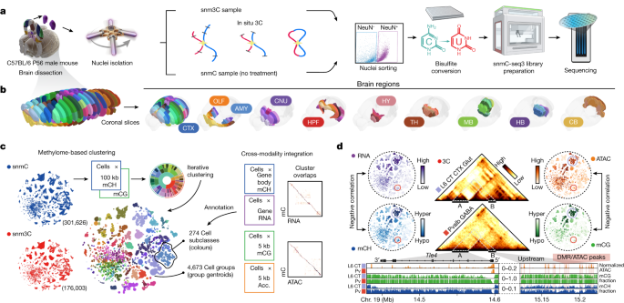
The second stage was genomic analysis, for which we used a pseudo-bulk-by-base tensor for mC, called base-resolution dataset (BaseDS), and a pseudo-bulk-by-2D-genome tensor for 3C, termed cooler dataset (CoolDS), to perform methylome and chromatin conformation analysis at flexible genomic resolutions, as depicted in Figs. 4–6. These pseudo-bulk tensors were generated at cell-group (thousands of profiles) and subclass (hundreds of profiles) levels to support multiple cellular granularities required by different analyses.

To investigate the relationship between gene status and the surrounding chromatin conformation diversity, we first performed quantile normalization along subclasses using the Python package qnorm (v.0.8.0)88 to normalize the transcript body mCH fractions and contact strengths of highly variable interactions. If any anchor of the interactions had been found next to the gene body, we used the transcript body’s mCH fraction to calculate thePCC. Similar to the domain boundary correlation analysis, we shuffled the contact strengths and mCH fractions within each sample and used the shuffled matrix to calculate null distribution and estimate FDR. FDR 0.001 is a significant correlation.

We used the imputed cell-level contact at the 10-kb resolution to perform the highly variable interaction analysis, for which the interaction represented one 10 kb-by-10 kb pixel in the conformation matrix. We filtered out any interactions that had one of the anchors overlapping with ENCODE blacklist (v.2)75. We then performed ANOVA for each interaction to test whether the single-cell contact strength of that interaction displayed significant variance across subclasses. The overall variability of the interaction across the brain was represented by the F statistics. We used F > 3 to cut off highly variable contacts, which was chosen after we looked at the contact maps and met the FDR criteria. ANOVA was only performed on interactions for which anchor distance was between 50 kb and 5 Mb, given that increasing the distance only led to a limited increase in the number of significantly variable and gene-correlated interactions (Extended Data Fig. 10b).

We used the imputed cell-level contact matrices at 25-kb resolution to identify domain boundaries within each cell using the TopDom algorithm89. We first filtered out the boundaries that overlapped with ENCODE blacklist (v.2)75. The boundary probability of a bin was defined as the proportion of cells having the bin called a domain boundary among the total number of cells from the group or subclass. The contingency table is used to identify the differential domain boundaries between n cell subclasses. The number of cells in a group that have a bin called a boundary or not is represented by the values in each row. We computed the Chi-square statistic and P value for each bin and used FDR < 1 × 10–3 as the cut-off for calling 25-kb bins with differential boundary probability.

Both snmC-seq and snATAC dataset 11 have the same dissection tissues. We utilized this experimental design to integrate cells from the mC and ATAC datasets within each major region. Of note, the snmC-seq data were enriched for NeuN+ by FANS, whereas the snATAC data unbiasedly profiled all cells. Therefore, we also separated neurons from non-neuronal cells and IMNs to balance the integration, especially in the first round. The integration was done using the mCg hypomethylation score and 5-kb bins. The stop criteria and cluster assignment were similar to the mC–RNA integration method. The alignment score was calculated using either k or 20 cells if the dissection region is larger. All ATAC cells assigned to each mC cell group have been combined to create the matched accessibility profile.

Source: Single-cell DNA methylome and 3D multi-omic atlas of the adult mouse brain

Downsampling of mC and RNA using the TF-IDF transformed matrices: Application to CCVs

CCA was also performed with the downsampling framework using 100,000 cells from each dataset as a reference and the others as query, but taking the TF–IDF transformed matrices as input. The reference cells were projected to the same space as the query cells. B_rmm_rm Ref were converted to. Then ({{B}{{\rm{m}}}}{{\rm{qry}}}) and ({{B}{{\rm{a}}}}{{\rm{qry}}}) were converted to ({{X}{{\rm{m}}}}{{\rm{qry}}}) and ({{X}{{\rm{a}}}}{{\rm{qry}}}), respectively, with TF–IDF using the IDF of reference cells, and the CCVs (denoted as ({U}{{\rm{qry}}}) and ({V}{{\rm{qry}}})) were computed using ({U}{{\rm{qry}}}={X}{{{\rm{m}}}{{\rm{qry}}}}({X}{{{\rm{a}}}{{\rm{ref}}}}^{T}{V}{{\rm{ref}}})/S) and ({V}{{\rm{qry}}}={X}{{{\rm{a}}}{{\rm{qry}}}}({X}{{{\rm{m}}}{{\rm{ref}}}}^{T}{U}{{\rm{ref}}})/S). Aligning and locating anchors are the next steps. It was the same thing as integrating the mC and RNA data.

$${{X}{{\rm{a}}}}{ij}=\log ({{{\rm{T}}{\rm{F}}{\rm{r}}{\rm{e}}{\rm{q}}}{{\rm{a}}}}{ij}\times \mathrm{100,000}+1)\times {{\rm{I}}{\rm{D}}{\rm{F}}}_{j}$$

$${{{\rm{T}}{\rm{F}}{\rm{r}}{\rm{e}}{\rm{q}}}{{\rm{a}}}}{ij}=\frac{{{B}{{\rm{a}}}}{ij}}{\mathop{\sum }\limits_{{j}^{{\prime} }\,=1}^{{\rm{No.}}\,{\rm{bins}}}{{B}{{\rm{a}}}}{{ij}^{{\prime} }}}$$

X_ij’slog (rmTrmFrmrrmemq_ij’s times) The embedding of single cells U was then computed using singular value decomposition of X, where (X=US{V}^{T}). We use the LSI model to derive Um. The intermediate matrices S and V and vector IDF were used to transform the ATAC data Ba to Ua, by

The embedding was calculated using LSI with log term frequencies. The conversion of the matrix B to X was done by dividing the row sum of the matrix into two fractions, one for term frequencies and one for inverse frequencies.

PCA on gene-body signals was insufficient to capture the open chromatin heterogeneity in snATAC-seq data10,30. Latent semantic indexing (LSI) applied to binarized cell-by-5-kb bin matrices had demonstrated promising results for snATAC-seq data embedding and clustering30. To align snATAC-seq data with snmC-sque data at a high resolution, we developed an extended framework based on approach 30.

The original CCA framework of Seurat (v.3) is difficult to scale up to millions of cells owing to the memory bottleneck, whereby the mC cell-by-RNA matrix was used as the input to CCA. We randomly selected 100,000 cells from every dataset and transformed them into a reference that we could fit in the CCA. Specifically, the canonical correlation vectors (CCVs) of ({X}{{\rm{ref}}}) and ({Y}{{\rm{ref}}}) (denoted as ({U}{{\rm{ref}}}) and ({V}{{\rm{ref}}}), respectively) were computed using ({U}{{\rm{ref}}}S{V}{{\rm{ref}}}^{T}={X}{{\rm{ref}}}{Y}{{\rm{ref}}}^{T}), where ({U}{{\rm{ref}}}^{T}{U}{{\rm{ref}}}=I) and ({V}{{\rm{ref}}}^{T}{V}{{\rm{ref}}}=I). Then the CCV of ({X}{{\rm{qry}}}) and ({Y}{{\rm{qry}}}) (denoted as ({U}{{\rm{qry}}}) and ({V}{{\rm{qry}}}), respectively) were computed using ({U}{{\rm{qry}}}={X}{{\rm{qry}}}({Y}{{\rm{ref}}}^{T}{V}{{\rm{ref}}})/S) and ({V}{{\rm{qry}}}={Y}{{\rm{qry}}}({X}{{\rm{ref}}}^{T}{U}{{\rm{ref}}})/S), respectively. The embeddings from the reference and query cells were concatenated for anchor identification.

We applied the framework to all subclasses of the mouse brain and cell clusters. The combination of the two sources of DMRs captured CpG fraction diversity in a variety of cell types. There were around 10 million unique yet overlapping DMRs after the combination. We then merged the DMRs to obtain a final non-overlapping DMR list (bedtools merge -d 0), which included 2.56 million DMRs. The data availability section reports all the overlap and non-overlapping DMRs. In the subsequent analysis, when DMR was used to calculate correlation or scan motif occurrence, we started with the 10 million overlapping DMRs. We selected the DMR with the strongest value (that is, most significant PCC or highest motif score) among the overlapping ones. The DMRs in the final results were non-overlapping.

For each clustering round, we assessed whether a cluster required additional clustering in the next iteration based on two criteria: (1) the final prediction model accuracy exceeded 0.9, and (2) the cluster size surpassed 20. In total, we executed four iterative clustering rounds, which produced the following cluster numbers: 61 (L1), 411 (L2), 1,346 (L3) and 2,573 (L4). We further separated cells within L4 clusters in the final round by considering their brain dissection region metadata. We decided to combine dissection regions with smaller numbers of cells with their closest ones based on the average distance between the PC space of L4 clustering. The final cells had clusters and dissection regions. Incorporating dissection region data, which offered insights into the physical location of a cell, enhanced the flexibility of the analysis, such as enabling spatial region comparisons. Furthermore, we acknowledged that generating pseudo-bulk profiles from cell-level data demanded substantial computational resources. Combining cells at the subclass level during subsequent analyses was initially easy because they were aggregation cells at a higher granularity.

The model on test data achieved a specified accuracy during the iterative process of merging and training, with an accuracy of.95) for the first round. The variation of cluster membership as random seeds changed was influenced by the resolution parameter. Therefore we used relatively small resolution values during each clustering stage (0.25 for the first iteration, 0.2–0.5 for the remaining iterations; the Scanpy default is 1). The approach reduced randomness and underestimated cluster numbers. Any under-split clusters that were further delineated in the subsequent rounds were the result of four rounds of iteration. This framework was incorporated in ALLCools.clustering. ConsensusClustering.

Source: Single-cell DNA methylome and 3D multi-omic atlas of the adult mouse brain

t-SNE and UMAP79 Principal Components for Large-Scale Cell-by-Cluster Analysis in a Cloud Environment

Calculate principal components (PCs) in the selected cell-by-CEF matrices and generate the t-SNE78 and UMAP79 embeddings for visualization. t-SNE was performed using the openTSNE80 package using previously described procedures81.

Both the snmC and snm3C datasets were analyzed. The first was a four-step process. The cells that were found in the pre-clusters contained potential doublets or low-quality cells. We started with all cells passing the primary QC filters and used the plate-normalized cell coverage (PNCC) metric to mark problematic pre-clusters. The average final reads of cells in the same plate were used to calculate the metric. We reasoned that cells at the same plate underwent all the library preparation steps inside the same PCR machine, thereby sharing the closest batch conditions. We observed some pre-cluster aggregating cells mostly showing extreme PNCC values (<0.5-fold or >2-fold) compared with most other clusters, which is a hallmark of problematic cells (Extended Data Fig. 2i). For each pre-cluster, we did a permutation-based statistical test to determine the abnormality. We randomly sample null-population cells with the cluster size, and then we divided the sample on a 10,000 time basis. We then calculated P values for the observed PNCC mean (two-tailed test, larger or smaller) and standard deviation (s.d., one-tailed test, larger) compared with the null PNCC mean and s.d. distribution. The FDR was calculated using a procedure called the Benjamini–Hochberg procedure72 which marked the pre-clusters as low-quality. There were 8,979 snmC and 737 snm3C cells removed from further analyses.

The large tensor dataset was chunked and compressed into Zarr format66, and stored in the object storage of the cloud platform. Data analysis was done using three packages. SkyPilot package69 was used to set up cloud environments, whereas the SnakeMake package65 was used to facilitate large-scale computation. Additionally, the ALLCools package (v.1.0.8) was updated to perform methylation-based cellular and genomic analyses, and the scHiCluster70 package (v.1.3.2) was updated for chromatin conformation analyses. In the Data and Code availability sections, we provide information for these tensor storage and reproducibility-related details (package version, analysis notebook and pipeline files). For simplicity, the description below focused mainly on key analysis steps and parameters.

Primary QC for DNA methylome cells included the following criteria: (1) overall mCCC level of <0.05; (2) overall mCH level of <0.2; (3) overall mCG level of >0.5; (4) total final reads of >500,000 and <10,000,000; and (5) bismark mapping rate of >0.5. Note that the mCCC level estimates the upper bound of the cell-level bisulfite non-conversion rate. Additionally, we calculated lambda DNA spike-in methylation levels to estimate the non-conversion rate for each sample. All samples demonstrated a low non-conversion rate (<0.01; Extended Data Fig. 2i). We used loose cut-offs to prevent potential cell or cluster loss in the primary filtering step. The clustering-based QC described below accessed potential doublets and low-quality cells. For the 3C modality in snm3C-seq cells, we also required cis-long-range contacts (two anchors >2,500 bp apart) >50,000.

The Salk Institute approved all of the procedures using live animals. The adult mice were purchased from the Jackson Laboratory at 7 weeks of age and then kept for up to 10 days in the animal barrier facility. Brains were sliced and reassembled in an ice cold dissection buffer. According to the Allen Brain Reference Atlas CCF, brains were sliced at 600-m intervals from the frontal pole and 18 slices were obtained. The data is in an extended data fig. 1b) For all the snm3C-seq samples, brains were sliced coronally at 1,200 μm, which resulted in a total of 9 slices and dissected 2–6 combined brain regions according to the CCFv3 (Extended Data Fig. 1b). Each region was pooled from animals, and the biological replicas were processed per region. Supplementary Table 1 contains comprehensive brain dissection data. Predetermining sample sizes was not done using statistical methods. We empirically determined the use of two to three biological experiments for all single-cell epigenomic experiments to achieve minimum reproducibility for this large-scale project. The handling of the tissue samples did not involve blind and randomization. The regions were registered in CCFv3 at 25 m resolution using the ITK-SNAP60, which is available in the Data availability section.