Dynamic Interface Printing with a Motion System Based on GelMA, PEGDA, HDDA and NEMA 23 for In Situ Imaging
H.T. is an inventor of computed axial lithography (CAL), an additive manufacturing process that the authors of the article refer to and over which they assert Dynamic Interface Printing has several advantages. H.T carries out research, holds funding for CAL and holds a small amount of shares in a company that holds a licence to practiceCAL.
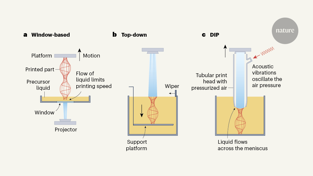
Fresh approaches to 3D printing can change the way objects are produced to serve a wide range of industries. A substantial and expanding category of 3D-printing processes — sometimes called digital light manufacturing — uses patterns of light projected onto a liquid resin to trigger the liquid to solidify at defined positions, thereby forming solid structures in desired shapes. The ultimate goal is to develop the processes to print features at larger scales by using a range of materials and at sizes suitable for industrial applications. Striking issues limit the speed of current processes and the quality of objects is reduced by the scattering of light patterns in liquid. Writing in Nature, Vidler and colleagues reported on a 3D-Printing strategy that could solve these problems.
To identify the ideal parameter space for DIP, a range of print speed and optical dose combinations were tested using three materials: PEGDA, GelMA and HDDA. Each combination has a triplicate with dimensions of 55 15mm3 printed, with successful outcomes being defined by the presence of a sharply delineated structure and smooth surface finish. Structures that did not meet these requirements, either because they were only partially resolved or because no structure had been produced, were removed from the parameter map. The print-speed parameters space was limited by the rate of new material that can wet the interface. Inadequate wetting typically caused the interface to fluidically ‘pin’ to the underlying structure as the polymerization rate exceeded the mass transport of new material.
A second system iteration was developed for in situ imaging, with modifications to allow the printing container to move relative to a stationary probe (Supplementary Fig. 3). The system incorporated a custom CoreXY motion system and a NEMA 23 ball-screw linear stage to translate the entire CoreXY stage relative to the stationary print head. The blue reflective mirror and a 50:50 beam splitter were used to illuminate in situ. Either a custom wellplate holder with a red collimated backlight was used for illumination. To maintain physiological temperatures and sterility during printing, the motion components and print head were enclosed within a custom heated chamber. Sterility was maintained by continuous HEPA filtration during printing, surface sanitization with 70% ethanol and sterilization with UV-C before use.
Direct volume manipulation of the air volume within the print head allowed for acoustic manipulation of the interface. The approach was easy to understand. The set-up consisted of a 3 inch 15 W voice coil driver (Techbrands, AS3034) affixed to an enclosed 3D printed manifold containing an inlet and outlet port (Fig. 3a and Supplementary Information section 2 and Supplementary Fig. 1c,d The voice coil was driven by a commercially available amplifier (Adafruit, MAX9744) using the supplied auxiliary port, with specified waveforms sent by the MATLAB GUI. When possible, there was a range between 1 and 500 hertz. It was easy to coordinate the acoustic modulator with the rest of the motion, optical and pressure control by specifying a WAVe for each degree of freedom.
Formation and mixing of gelMA and norbornene functionalized sodium alginate mixtures using the same protocol for each form of PEGDA
We followed the same protocol for each form of PEGDA used in the study. The required weight fraction was dissolved in the same volume fraction as the water and thoroughly mixed for 10 minutes. After 0.035 w/w% and 0.25% were added to the mixture it was stirred until complete dissolution. The materials were then stored in light-safe Falcon tubes until required.
Warming the mixture to 40C and stirring prepared a solution of 50 g of 1,6-hexanediol diacrylate and 500 liters of phenylbis (2, 4,6-trimethylbenzoyl) phosphine oxide. The Sudan I photo-absorber was added in various quantities to control the resolution. The materials were then stored in light-safe Falcon tubes until required.
GelMA was synthesized following a previously reported protocol56, yielding a degree of substitution of 93% (confirmed by nuclear magnetic resonance). A 10% w/v GelMA solution was prepared by dissolving a little GelMA in some cell culture media at a temperature of 37 C. The solution was maintained at 37 C until complete dissolution, after which 3.5 bags of Tartrazine and 25 bags of LAP were added. The mixture was stored in the biosafety cabinet until it was required in order for it to be sterilized.
Norbornene-functionalized sodium alginate was synthesized based on a previously reported protocol57. In short, 10 g of sodium alginate were dissolved in 500 ml of 0.1 M 2-(N-morpholino) ethane-sulfonic acid buffer (145224-94-8, Research Organics) and fixed to pH 5.0. Then, 2.90 g of N-hydroxysuccinimide and 3.11 g of 5-norbornene-2-methylamine were added. The pH was fixed at 7.5 with 1 M NaOH. The reaction was done at room temperature. The mixture was dialysed against the water. The 1H nuclear magnetic resonance determined the degree of norbornene functionalization. A 7% w/v sodium alginate solution was prepared by dissolving 1 g of the sodium alginate in 14.29 ml of phosphate-buffered saline solution. Next, a small amount of LAP and 2, 2′-(ethylenedioxy)diethanethiol was added to the salt solution and mixed until it was. The pH was adjusted with 1 M NaOH until the solution was visibly opaque.
A solution of 50 mg of phenylbis(2,4,6-trimethylbenzoyl) phosphine oxide (511447, Sigma) and 5 g of diurethane dimethacrylate (436909, Sigma) was prepared by warming the mixture to 45 °C and stirring for 30 min. To remove trapped air bubbles, the mixture was transferred to a light-safe Falcon tube and centrifuged at 4,000 rpm for 10 min to remove residual air bubbles.
Source: Dynamic interface printing
Cell-Viability Determination with a Low-Density LCD Image Capsule over HDMI using the Freestyle System
A preliminary determination of cell viability was achieved using human embryonic cells from the Freestyle system. A cell solution with 7.2 million cells per deci litres was used for both the model of a kidneys and the cell-viability measurement. To determine cell viability a thin 500 m wall was printed and imaged using a live/dead viability/toxicity kit. Three structures were printed (n = 3), and measurements were taken after 24 h to determine the preliminary viability of the technique. Cell viability was determined at three locations for each sample (s = 3), with the total viability being an average of all collection points (Supplementary Fig. 18).
The three-dimensional design models of the capsule were created using nTop. A number of models were downloaded from Thingiverse.com. The slt file for each geometry was cut from it using Chitubox. As the frame rate of the HDMI signal was limited to 120 frames per second (fps), we commonly used projection frame rates that matched the acoustic driving frequencies to minimize motion blurring. The object was discretized into a voxel array according to the desired linear print speed and frame rate. The layer height (Lh) was determined as ({L}{{\rm{h}}}={v}{z}/f), where vz is the linear print speed and f is the acoustic excitation frequency, which matched the projection frequency. The image stack was further corrected using the convex-slicing algorithm to produce a secondary optimized image stack, with the sequence being sent to the projector over HDMI using Psychtoolbox-3 (ref. 58). The print sequence started by moving the print head to a defined distance above the print surface (or high-density material). The interface was connected to the image plane by means of a print head. The GUI had to control the location of the air–liquid interface by controlling the pressure, acoustic driving, and translation location in order to turn on theLED module. The optical power of the projection module was automatically set depending on the selected print velocity using the parameter space matrix. The printed structures were removed from the print volume and washed with alcohol. The excess material for soft structures was gently removed using a pipette, and resuspended in deionized water or cell culture media to remove unpolymerized material. The structures were detached from the container and kept in an appropriate solution.
The tool developed to correct for geometrical discretization differences between a traditional flat construction surface and a curved surface is called the convex-slicing algorithm. A detailed explanation of the convex-slicing process is given in the Supplementary Information. However, the main components will be briefly restated here. The Laplace pressure difference was determined using the Young–Laplace equation. Here, we used axisymmetric print containers such that (\hat{n}) can easily be found by substituting the general expressions for principal curvatures. The capillary length (l=\sqrt{\gamma /\rho g}), where γ is the material surface tension, ρ is the material density and g is the acceleration due to gravity, was used to normalize the radial and vertical coordinates of the interface as (x=r/l) and (y=z/l). The ordinary differential equation for the interface shape was x and y.
This equation can be readily solved using numerical integration with appropriate boundary conditions (Supplementary Information section 4). However, using this method would require numerical integration for the steady-state case, and moreover, we would need to solve each intermediate state during compression with the associated boundary conditions. We, instead, opted to approximate the solution using cubic Bézier curves for the steady-state case and approximating the compressed profiles by geometrically deforming the Bézier curve while ensuring volume equivalency (Supplementary Information section 7). This is computationally faster given the large number of intermediate surfaces within the transient region. The half-profile was centered on the printed head’s central z axis in order to convert the 2D Bézier solution into a 3D surface. This produced a sequence of surfaces starting at the compressed state and transitioning to the steady-state interface profile. The corresponding convex projection(s) were determined by minimizing the Euclidean distance between the Cartesian voxel grid and the surface arrays (Supplementary Information section 6). Reconstruction accuracy was validated by ‘replaying’ the projections over an empty voxel array and computing the Jaccard index between the reconstructed voxel array and the input voxel array (Supplementary Information sections 8 and 9).
To determine our theoretical optical model (Supplementary Information section 10), we employed a similar approach to Behroodi et al.59, who modelled the in-plane resolution as the spatial convolution of the point spread function (({\rm{PSF}}(x,y))) and the micro-mirror spatial arrangement ((f(x,y))), where (f\left(x,y\right)\ast {\rm{PSF}}\left(x,y\right)={\int }{-\infty }^{\infty }{\int }{-\infty }^{\infty }f({\tau }{1},{\tau }{2})\,\cdot \,{\rm{PSF}}\left(x-{\tau }{1},y-{\tau }{2}\right)\,{\rm{d}}{\tau }{1}\,{\rm{d}}{\tau }{2}), and τ1 and τ2 represent spatial shifts, summed over all possible displacements, during convolution. A transmissive efficiency is described by the relative angle of the ray incident and the amount of time it took for it to travel across the meniscus. Here, n1 and n2 represent the refractive index of the air and liquid, respectively, and (\hat{{\bf{u}}}) is the normal vector at a given point on the meniscus’s surface. The energy intensity along the transmissive vector ({\gamma }{z}) was approximated as a material-dependent Beer–Lambert decay ({\mathcal{H}}({{\boldsymbol{\gamma }}}{x},{{\boldsymbol{\gamma }}}{y},{{\boldsymbol{\gamma }}}{z})\,=\,\eta ({n}{1},{n}{2},\hat{{\bf{u}}},\hat{{\bf{n}}})\cdot \hat{{\bf{E}}}\,\exp \left(\frac{-{{\boldsymbol{\gamma }}}{z}}{{\varepsilon }{{\rm{d}}}\left[D\right]+{\varepsilon }_{{\rm{i}}}\left[S\right]}\right)) (Supplementary Information section 11), where, εd and εi are molar absorption coefficients of the photoinitiator and the light absorber, respectively, and D and S are the concentrations of the photoinitiator and light absorber of the photopolymer resin, respectively. The effectiveresolution depends on the height of the meniscus in relation to the focal plane. We mapped the coordinate of the focal plane and the corresponding coordinate on the surface of the meniscus, which produced a map of the effective size across the interface. The map was used to guess the accurate area fraction based on print head size and material properties.
To understand the formation of acoustically driven capillary-gravity waves, we used many established analytical approaches that describe the induced velocity and secondary streaming effects32 created by the meniscus (Supplementary Information sections 13–15). This analysis establishes the rules for capillary-gravity waves that are dependent on whether or not the effects are capillary or gravity-driven. The dispersion relation for capillary waves, ({\omega }^{2}=\frac{\gamma }{\rho }{k}^{3}+{gk}), relates the wave frequency (ω) to the wavenumber (k). The dominance of surface tension and acoustic parameters on the flow magnitude is linked to the unitless quantity “(lambda /l_rmcap)2” Here, lcap denotes the capillary length of the material. Thus, the flow velocity U scales as (U\propto \frac{{h}{0}^{2}\rho g\phi }{\lambda \mu }) for ((\lambda /{l}{{\rm{cap}}}) > 1) and (U\propto \frac{{h}{0}^{2}\gamma \phi }{{\lambda }^{3}\mu }) for ((\lambda /{l}{{\rm{cap}}}) < 1), where, h0, ϕ and μ represent the surface perturbation, wave amplitude and viscosity, respectively. The material and acoustic parameters are shown in the supplementary fig.
PIV was employed to understand the 3D flow field produced below the air–liquid boundary under acoustic excitation. A high-speed camera was used to capture the footage of 20-50 m poly. Particles are normal and orthogonal to the air–liquid boundary. PIVLab was used to perform particle tracing and velocity reconstruction. The exact parameters and methodology used can be found in Supplementary Information section 18. The velocity profiles for top-down and side are shown in Fig. 3c–e and Supplementary Figs. 8 and 9.
To determine the transient interface restabilization in the bulk flow, high-speed photography under a uniform backlight was captured at 5,000 fps (Supplementary Fig. 7). By segmenting the edge of the meniscus, we could track where the video stream was and determine restabilization. The time was determined by applying an exponential criterion which took into account the starting amplitude.
The material influx rate with and without acoustic excitation was determined by filling a glass cuvette with materials doped with black dye to prevent light transmission. The cuvette was placed on top of a red backlight, such that when the air–liquid boundary formed against the base of the cuvette, the transmitted light was observed by a CCD (Supplementary Information section 19). The material influx rate was measured by raising the air–liquid boundary with and without acoustic excitation and tracking the influx of dyed material which occluded the backlight transmission.
Source: Dynamic interface printing
Micro-Computational Tomography of Hydrogel Samples Using a Phoenix Nanotom M Scanner and a Zeiss NanoFab
Micro computed tomography images were acquired using a Phoenix Nanotom M scanner (Waygate Technologies, voxel size of 10 µm3, 90 kV tube voltage, 200 µA tube current and 8 min scan time). For hydrogel samples, the structures were briefly dried with tissue paper and mounted into a Falcon tube for imaging. The plastic cap on which the structures were placed provided a contrast between the printed structure and the supporting medium. Keyshot 11 was used to make the final micro computed tomography representation.
The images were taken with a 4 or a 10 objective. The large-format image was created using the images of larger constructs that were bigger than the field of view. Once the fluorescence images were acquired, cell-counting was performed on each live/dead image pair using a custom MATLAB script.
There are images of a scanning electron microscope on the FlexSEM 1000. Printed structures on glass slides were mounted directly on the microscope stage with no further sample preparation. The samples did not have a conductive coating applied. The electron microscope was operated in variable-pressure mode at 50 Pa. Images were acquired with a 15 keV beam using the ultra-variable detector. The field of view for the large structures needed a 40- to 50-millimeter working distance and several images were collected in a tiled manner and stitched together in postprocessing.
Helium-ion microscopy images were acquired with a Zeiss NanoFab using a helium source. During imaging, the flood gun was used to actively neutralize the surface, thus removing the need for a conductive coating. All structures were imaged using an accelerating voltage of 30 kV, a beam current of between 1 and 2 pA, and a field of view of 1,100 µm. Structures were printed directly onto a silanized glass slide and were mounted on the stage using the integrated mounting clips. Several images were taken and subsequently stitched using ImageJ/Fiji to facilitate the capture of larger structures.