Disynaptic Pathways as Markov Chains: Supplementary Data 3-5 Using the Ellipse Approximation

In Supplementary Data 3–5, these maps are defined using Pab rather than Wab, to facilitate comparison with the probability maps for disynaptic pathways defined below.

The normalization is with respect to the number of cells ({|B|}) of type B, because the connectivity map is defined as the average number of synapses received by a B cell from A cells, if the origin of the coordinate system is placed at the B cell.

Oit and the type-to-cell connecting matrix Itj are the output features of cell i.

It can be deduced from the matrix Pab that it is a Markov chain. The walker chooses a random input sphinx of the present neuron, then crosses the sphinx in a retrograde direction to reach the presynaptic stage. Then Pab denotes the probability of stepping from neuron b to neuron a.

The next-nearest neighbours, which are (sqrt2) lattice constant away, are pointed out by the orthogonal directions. The hexels were grouped by their q p, q or p. The resulting coordinate was in units of lattice constant (\times \sqrt{3}/2).

The ellipse approximation gives a parametric estimate of receptive field size. For a non-parametric estimate, I also used 1D projections onto directions defined on the hexagonal lattice. Each hexel was given coordinates (p, q), with the origin placed at the anchor location used for alignment.

The Width of the Maximum in a Gaussian Hexagon II: Corrections to the Wave Function and the Length of a Column

The above has implicitly defined (2\sigma ) as the width of a 1D Gaussian distribution, for which ({\sigma }^{2}) is the variance. This is the full width of the maximum. The width can be estimated at half-maximum, (sigma 2sqrt2 Mathematicsrmln2approx 2.4sigma ). For either estimate, the width is proportional to (\sigma ). I stick with the simpler estimate (2\sigma ), which can be readily scaled by any multiplicative factor of the reader’s preference.

The first term of the covariance matrix C effectively regards the probability distribution as a weighted combination of Dirac delta functions located at the lattice points. If each Delta function is replaced by a uniform distribution over the corresponding hexagon, the second term is a correction. This replacement is biologically relevant because a column receives visual feedback from a non zero solid angle. Without the correction, the length and width would vanish if the image consists of a single hexel concentrated at a single delta function. The width and length of an image are changed with a single non-zero hexel. The correction becomes relatively minor when the length and width of the image are large.

The length of the hexagon side is indicated by the 2 2 identity matrix and s. The length and width of hexel is defined as 2.sigma _max and 2.sigma _min. The approximating ellipse is centred at the image centroid, and oriented along the principal eigenvector of the covariance matrix.

Comparative Analysis of Two Types of Connected Cells in an Adult Drosophila Brain: v783 and Fig. 3c

This work is based on v783 of the proofread reconstruction of an adult female Drosophila brain15,16,17. All connections are drawn from the right side of the eye. Companion papers present cell-type annotations of the boundaries of the brain, as well as the cells that lie in the optic and central brain.

Another approach to interpretability is to look at low-dimensional projections of the 2T-dimensional feature vector. For each cell type, we select a small subset of dimensions that suffice to accurately discriminate that type from other types (Extended Data Fig. 3c). The elements of the feature are normalized so that they reflect the input and output portion of the equation. The total number of all inputs and outputs is also known as the denominator in these quantities.

Dm3p and Dm3q are similar to each other than to Dm3v, and TmY9q and TmY9q are almost identical to each other. Whether similarity of connectivity corresponds with transcriptomic similarity remains to be seen.

Stochastic microscopy of Dm3, TmY4 and LC10: the motion pathway to line amacrine cells

Strausfeld wrote Golgi studies of calliphora and Eristalis1, as well as Musca65. Strausfeld also mentioned unpublished observations of line amacrine cells in Locusta and Apis1. There is a Golgi study of a line amacrine cells.

Light microscopy with multicolour stochastic labelling3 went beyond Golgi studies by splitting Dm3 into two types with dendrite at orthogonal orientations. The transcriptomes of both Dm3p and Dm3q differed prior to adulthood. (Ref. 18 used the alternative names Dm3a and Dm3b.) Immunostaining showed that Dm3q expresses Bifid, whereas Dm3p does not. Ref. 18 also analysed a reconstruction of seven medulla columns64, with the results showing that Dm3p and Dm3q prefer to synapse onto each other, foreshadowing the present work, and speculatively placed Dm3 cells in the motion pathway.

TmY4 and TmY9 have been described before. The two TmY9 types can be distinguished by the tangential directions of their neurites (Fig. 2b,c), or by their connectivity (Fig. 3a, and Extended Data Figs. 4 and 5). Their profiles are slightly different. TmY9q only works in layer 1 and 2 of the lobula plate. In the lobula, layers 5 and 6 are frequently bistratified, whereas layer 9 is often monostratified.

LC10 cells project from the lobula to the anterior optic tubercle12, and have been linked with visually guided courtship behaviours66. The four LC10 types were identified using GAL4 transgenic lines and their stratification was done in the lobula13. Using the connectomic approach described in a companion paper4, I identified a fifth type (LC10e), which stratifies in layer 6 of the lobula. LC10e was further subdivided into two groups on the basis of connectivity. The two groups are separated by a body of water.

My conjecture that LC10e detects a corner or T-junction is specific to the ventral variant, which receives strong input from TmY9q and TmY9q⟂. The ventral visual field is expected to be more important for form vision, assuming that the fly is above the landmarks or objects to be seen.

FlyWire provides predictions of neurotransmitter identity that are based on the electron micrographs67. TmY4 is predicted to becholinergic whereas Dm3 is predicted to be glutamatergic. The same information can be drawn from the expression of neurotransmitter synthesis and transport genes.

Whether a neurotransmitter has an excitatory or inhibitory effect on the postsynaptic neuron depends on the identity of the postsynaptic receptor. The fly brain69 has a postsynaptic receptors that’s nicotinic, which makes Acetylcholine excitatory. Glutamate is inhibitory in Drosophila when the postsynaptic receptor is GluClα70.

On the hemibral lattices of the Li11, Li18, Li12, and LPi07: predictions from electron micrographs

According to transcriptomic data Dm3 expresses GluCl. Unpublished data indicate that TmY4 and TmY9 also express GluClα (Y. Kurmangaliyev, personal communication). Dm3p and Dm3q contain transcriptomic information, but not Dm3v.

The prediction of what the two LPi15 and14 will be is based on electron micrographs16,67. LPi07 cells are predicted to be GABAergic, glutamatergic or uncertain on the basis of electron micrographs, and are presumed to be inhibitory.

Some of the hexagonal lattices are drawn in the figure as if they are uniform. The drawings are intended to portray only the nearest-neighbour relations of cells and columns, and do not accurately represent distances. The lattices were constructed in a more accurate way, which was used to show how lattice properties vary in space for the right and left brains of some flies. Visual acuity also varies across the retina in flies and other insects52,77.

Our new names placeleading zeros in the way of colliding with Li1 and Li26 The hemibrain names Li11 to Li20 and mALC1 and mALC29 have been used by few or no publications, so there is little cost associated with name changes. In any case, we were only able to establish conclusive correspondences for a minority of the hemibrain Li11 to Li20 types, which are detailed in Supplementary Data 1. Hemibrain Li16 is now Li28, a pair of full-field cells. Hemibrain Li11 was split into Li25 and Li19 (see the ‘Morphological variation’ section). Hemibrain Li18 was split into three types: (1) Li08 covers the whole visual field. (2) Li04 covers a dorsal region except for the dorsal rim. It is tangentially polarized, with the axon more dorsal than the dendrites. Both axon and dendrite point in the posterior direction, perpendicular to the direction of polarization. The axon is thinner than the dendrites. (3) Li07 has ventral coverage only. The axons are in one layer, and extend over a larger area than the dendrites, which hook around into another layer and are mostly near the ventral rim. We thought about combining Li03 and Li06, but they are quite different. Li07 would merged with Li08 before Li04 in a hieratic clustering.

The v796 reconstruction included 745 Tm1, 746 Tm2, 716 Tm9, 796 Mi1, 749 Mi4, 730 Mi9, 715 L1, 763 L2, 709 L3 and 743 L5 cells. These numbers are smaller than the total number of cells proofread in v783 (ref. 4), but the deficit is generally less than 10%.

Mi1 cells were assigned automatically to hexagonal lattice points. Locations of L cells were assigned by placing them in one-to-one correspondence with Mi1 cells using the Hungarian algorithm applied to the connectivity matrix. The locations of other hexel types were assigned by placing them in one-to-one correspondence with L cells again with the Hungarian algorithm.

Supplementary Data 2 shows the locations of hexel types in (p, q) coordinates. Following the convention defined in ref. 29, all three cardinal axes of the hexagonal lattice point upwards (Fig. 1f). The vertical axis is directed dorsally. The anterodorsal and posterodorsal directions are used for the p and q axes. The hexagons of the lattice are oriented with flat sides at the top and bottom of them, as well as pointed tips at the left and right. The p–q axes are related to the dorsoventral and anteroposterior axes in a different way.

The figures show the lattice of columns. The lattice is left inverted relative to the medulla columns thanks to the optic chiasm. Therefore, back-to-front motion on the retina is front-to-back motion on the medulla lattice. In other words, the p and q axes are swapped in the eye relative to the medulla. The p and q axes are very close to one another in the medulla, which is situated along the anteriorposterior direction. The p and q axes are closer to 120° apart in the eye, where the ommatidia more closely approximate a regular hexagonal lattice.

How accurate is it to discriminate between intrinsic and boundary types in an x-ray lattice? I: Type assignments and the differentiation of the Pm family

I would run from 1 to N points of a hexagonal lattice if the image had hexel values (h_i) at Cartesian coordinates. Normalizing the image yields a probability distribution ({p}{i}={h}{i}/({\sum }{j=1}^{N}{h}{j})). Then compute the coordinates of the image centroid by

C is forlimits_i and is divided into two parts, one beginning and one ending.

It was sufficient for the feature dimensions to have only intrinsic types. This leads to the same results if features are including both boundary types and T > 700.

The sums are all over the brain. If neuron i is a cell intrinsic to one optic lobe, the only nonvanishing terms in the sums are due to the intrinsic and boundary neurons for that optic lobe.

On the basis of the auto-correction procedure, we estimate that our cell type assignments are between 98% and 99.9% accurate. For another measure of the quality of our cell typing, we computed the ‘radius’ of each type, defined as the average distance from its cells to its centre. Here we computed the centre by approximately minimizing the sum of Jaccard distances from each cell in the type to the centre (see the ‘Computational concepts’ section). A large type radius can be a sign that the type contains dissimilar cells, and should be split. Almost all of the final types lie below 0.6. 3b). Lat has a high type that should be split into two parts. The type radii are essentially the same, whether or not boundary types are included in the feature vector (data not shown).

Discriminators for all types are available in Supplementary Data 4. Many although not all discriminations are highly accurate. Discriminative features include both intrinsic and boundary types.

The Pm family can be seen in the two-dimensional space of C3 input fraction and TmY3 output fraction. In this space, Pm04 cells are well-separated from other Pm cells, and can be discriminated with 100% accuracy by ‘C3 input fraction greater than 0.01 and TmY3 output fraction greater than 0.01’. This conjunction of two features is a more accurate discriminator than either feature by itself.

Clustering metrics and exact clustering: Precision, recall, F-score, and precision splitting of subject type data with arbitrary boundary types

We also measured the drop in the quality of predicates if excluding boundary types (where the predicates are allowed to contain intrinsic types only). As is the case with the clustering metrics, the impact on predicates is marginal (weighted mean F-score drops from 0.93 to 0.92).

Every type has its own process for calculating precision, recall and F-score, and it consists of all possible combinations of input type inputs and outputs. A few optimization techniques are used to speed up this computation, by calculating minimum precision and recall thresholds from the current best candidate predicate and pruning many tuples early.

Each type consists of 2 input types and output types, which make up an optimal predicate. Both tuples are limited to size 5 and are ideal for predicting the subject types, defined as follows:

True positive predictions that are actually of type T are used to calculate precision.

The centre of each type was estimated using the element-wise trimmed mean after we arrived at the final list. Then, for every cell, we computed the nearest type centre by Jaccard distance. The nearest type centre was associated with 98% of the cells. Some disagreements were reviewed manually. In the majority of cases, the annotators were correct, but sometimes they were wrong. The remaining cases were mostly attributable to proofreading errors. There were some cases in which the type centre was contaminated by human-misassigned cells, which resulted in more mis assignment by the algorithm. After addressing these issues, we applied the automatic corrections to all but 0.1% of cells, which were rejected using distance thresholds.

We used computational methods to split types that could not be properly split in stage 2. Some candidates for splitting (such as Tm5) were suggested by the image analysts. Some candidates were suspicious because they contained so many cells. Finally, some candidates were scrutinized because their type radii were large. If the splits are in line with the tiling principle, we accept them, even if they are not aligned with the average linkage that we applied.

Citizen scientists have created farms with all of the cells they’ve found. The farms showed where the cells were still found. If they found a bald spot, a popular method to find missing cells was to move the 2D plane in that place and add segments to the farm one after another in search of cells of the correct type. Farms also helped with identifying cells near to the edges of neuropils, where neurons are usually deformed. Having a view of all other cells of the same type made it possible to extrapolate to how a cell at the edge should look.

Citizen scientists created a comprehensive guide with text and screenshots that expanded on the visual guide. They also found and studied any publicly available scientific literature or resources regarding the optic lobe. They shared findings at discuss.flywire.ai, which as of 10 October 2023 had over 2,500 posts. Community managers shared their findings from the literature with citizen scientists, consulted specialists on Flywire and gave feedback.

The community resources fostered an environment for sharing ideas and information among members of the community. Community managers answered questions, provided resources and performed various functions in the community. Project progress was provided by daily statistics, which were shared on the discussion board. During the week there were live interaction, demonstrations, and solution solutions in the video streams led by the community manager. There are a number of ways in which citizen scientists are able to organize as a result of the environment created by these resources.

Source: Neuronal parts list and wiring diagram for a visual system

Connectomic Cell Approach to Type Detection: A Case Study in the Optic Lobes of an Eyewitness Citizen Scientist

The optic lobes are divided into five regions (neuropils): lamina of the compound eye (LA); medulla (ME); accessory medulla (AME); lobula (LO); lobula plate (LOP). There are two groups of cells in the regions with the skelps.

The top 100 players from Eyewire79 had been invited to proofread in FlyWire24. After 3 months of proofreading in the right optic lobe, they were encouraged to also label neurons when they felt confident. Many citizen scientists did a mixture of both. Sometimes they annotated cells after proofreading, and other times searched for cells of a particular type to proofread.

Our connectomic cell approach to typing is initially seeded with some set of types, to define the feature vectors for cells (Fig. 2a), after which the types are refined by computational methods. Our initial seeding relied on the time-honoured approach of cellular typing, sometimes assisted by computational tools. It is worth noting that ‘morphology’ is a misnomer, because it refers to shape only, strictly speaking. Orientation and position are actually more fundamental properties because of their influence on stratification in neuropil layers. Thus, ‘single-cell anatomy’ would be more accurate than morphology, although the latter is the standard term.

A connection probably doesn’t exist from other studies. For example, T1 cells lack output synapses26,78. Therefore, in our analyses, we typically regarded the few outgoing T1 synapses in our data as false positives and discarded them.

Another heuristic is to look for extreme asymmetry in the matrix. The number of connections from A to B may be much larger than from B to A. The reason is that the strong connection from A to B means the contact area between A and B is large, which means more opportunity for false-positive synapses from B to A. False-positive rates for synapses are estimated in the flagship paper24.

In the central brain, most cell types have cardinality 2 (cell and its mirror twin in the opposite hemisphere; Extended Data Fig. 1e). In the hemibrain, the cardinality is typically reduced to one. Therefore, whether there is a connection between cell type A and cell type B must be decided based on only two or three examples of the ordered pair (A, B) in all the connectomic data that is so far available. Given the small sample size, setting the threshold to a high value makes sense for false positives to be avoided.

In order to estimate the under-recovery, we must use themodular types29 which are defined as cell types that are in one-to-one correspondence with columns. A previous reconstruction of seven medulla columns identified 20 modular types28. These largely correspond to the cell types that contain from 720 to 800 cells in our reconstruction (Fig. 1d). The top end (800) of this range is probably the true number of columns in this optic lobe. The lower end of the range is 720, suggesting that under-recovery is usually less than 10%.

A genuine analysis of modularity requires going beyond simple cell counts, and analysing locations to check the idea of one-to-one correspondence. The analysis is not finished for the foreseeable future. We don’t commit to whether those types containing 720 or more cells are truly modular by applying the term “numerous” to them.

In the left eye area, there are approximately 38,500 intrinsic cells, 3,700 VPNs, 250 VCNs, 150 Heterolateral Cells and 5,000 photoreceptor cells. The tables comparing left/ right counts by superclass are available for download.

R7 and R8 contain 650 cells, while R1 and R6 contain 3,400 in version 783 of the FlyWire connectome. These numbers are not inconsistent with modularity because photoreceptors are especially challenging to proofread in this dataset and under-recovery is higher than typical.

An Effective Weighted Distance and Its Uses in Neuronal Parts List And Wiring Diagram for a Visual System. Part I: The Cost Function

$$J\left({\bf{x}},{\bf{y}}\right)=\frac{{\sum }{t}\min \left({x}{t},{y}{t}\right)}{{\sum }{{t}^{{\prime} }}\max \left({x}{{t}^{{\prime} }},{y}{{t}^{{\prime} }}\right)}$$

The weighted distance d is defined as a single minus the weighted similarity. The quantities are non negative since our features are non negative. In our cell typing efforts, we have found empirically that Jaccard similarity works better than cosine similarity when feature vectors are sparse.

This cost function is convex, as d is a metric satisfying the triangle inequality. Therefore, the cost function has a unique minimum. We used different methods to decrease the cost function.

Source: Neuronal parts list and wiring diagram for a visual system

Hierarchical Diagram for Neuronal Parts List and Wiring Diagram for a Visual System: Diagrams from Cytoscape 81

The trimmed mean was used for auto-correction of type assignments. This gave good robustness to the noise from false detections. For the type radii, we used a coordinate descent approach, minimizing the cost function with respect to each ci in turn. The loop included every i for which some xi was non-zero. This happened within a few loops.

Each cluster is generally a mixture of types from multiple neuropil families. Sceptics may think such mixing is caused by the noisiness at the large distances. The closest types tend to be from the same family. But plenty of dendrogram merges between types of different families happen at intermediate distances rather than the largest distances. Some of the different types from different families seem to have some connection to biology.

We used the Cytoscape 81 to draw the wiring diagrams. Hierarchical layout was used for two of the three figs. The layout tries to make arrows point in the same direction. After a diagram was generated, the nodes were manually shifted to minimize obstructions.

Source: Neuronal parts list and wiring diagram for a visual system

Boundary Neurons: Axons and a Family of Sm’s (Sm,Tlp) Types

Boundary neurons are those with at least 5% (and less than 95%) of synapses in the optic lobe regions, and are either visual projection, visual centrifugal or heterolateral neurons.

We used the term axe in the main text. An axon is defined as some portion of the neuron with a high ratio of presynapses to postsynapses. This ratio might be high in an absolute sense. The neuron’s dendrite may play a role in determining the ratio in the axon. In either case, the axon is typically not a pure output element, but has some postsynapses as well as presynapses. The obvious is that there is an axon, but we have made some judgement calls about it for certain types. The presence of varicosities can be seen in the axon, even if there isn’t a look at the sphinx. A dendrite has more postynapses to presynapses than an axon.

The axon–dendrite distinction does not hold, so an amacrine cell is defined as one for which the ratio of preSynapses and Postsynapses is the same throughout. The branches of the amacrine cell are commonly referred to as dendrites but the neutral term is more appropriate for avoiding confusion.

The Sm family more than doubles the number of medulla interneuron types, relative to the old scheme with only Pm and Dm. The Sm family might be related to the M6-LN class of neuron previously defined88. M6 is where Sm mainly occurs, so the correspondence is unclear. But some Sm types stratify at the border between M6 and M7, and therefore could be compatible with the M6-LN description.

A Tlp neuron projects from the lobula plate to the outside. Tlp1 to Tlp5 were defined first6, and Tlp11 to Tlp14 were defined later on10. We have identified some of them. The names of Tlp11, TLP12 and TLP13 should be retired as they can now be identified with Tlp5, Tlp1 and Tlp4 respectively.

Pm1, 1a and 26 were each split into two types. Pm3 and 4 are still defined. We additionally identified six new Pm types, for a total of 14 Pm types, numbered Pm01 to Pm14 in order of increasing average cell volume. The new names can be distinguished from the old ones by the presence of leading zeros. They are all predicted to be gybanergic. Pm1 was split into Pm06 and Pm04, Pm1a into Pm02 and Pm01, and Pm2 into Pm03 and Pm08.

LPi names were originally based on stratification in layers 1 to 4 of the lobula plate, including LPi1-2 and 2-110; LPi3-4 and 4-38; and LPi2b and LPi34-1210 (we are not counting fragments for which correspondences are not easy to establish). We have added nine new types for a total of 15.

stratification is no longer enough for naming now that the different kinds have become more common. Adding letters to differentiate between different cells could be done to save the naming system. It is possible to call themLPi15 andLPi05LPi1 andLPi1 andLPi1, where “f” and “s” mean full field and small. For simplicity and brevity, we instead chose the names LPi01 to LPi15, in order of increasing average cell volume. Correspondences with old stratification-based names are detailed in Codex.

The criteria were applied when we identified the large recurrent neurons. The neurons were intrinsic, so they met the rich- club criteria. Second, at least 50% of the neuron’s incoming connections were contained within the subnetwork of a single neuropil. Third, at least 50% of the neuron’s outgoing connections were contained within the same neuropil.

Tm5a, Tm5b and Tm5c were originally defined by single-cell anatomy and Ort expression7,50. Tm5a is cholinergic, the majority of the cells extend one dendrite from M6 to M3, and often has a ‘hook’ at the end of its lobula axon. Most cells extend from M6 to M3 and Tm5b is cholinergic. Tm5c is glutamatergic and extends its dendrites up to the surface of the distal medulla. Three of our types are consistent with these morphological descriptions (Fig. 7a), and receive direct input from inner photoreceptors R7 or R8.

In order for a neurons to be reached through directed pathways, it must be defined as a subnetworks. All neuron are reachable and ignored in the relaxed criterion of WCCs.

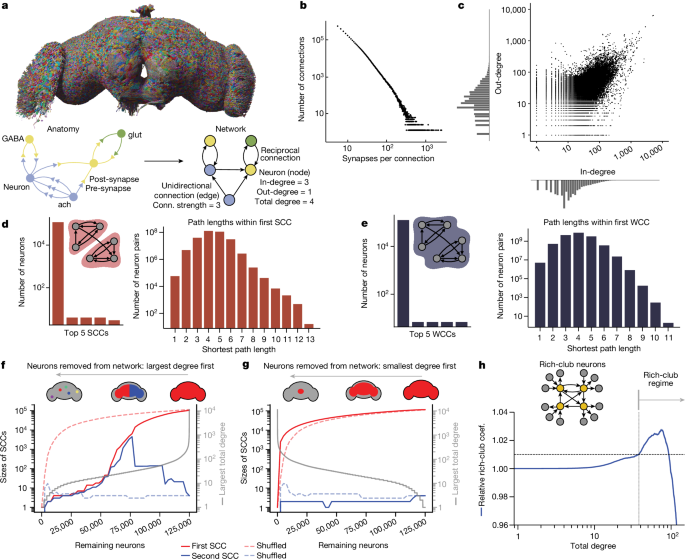
The in- and out- degree is the number of incoming and outgoing partners a given neuron has. The total degree of a neuron i is the sum of in-degree and out-degree:

We compared the statistics of various null models with those of the wiring diagram G(V,E). The simplest null model that we used was a directed version of the ER model ({\mathcal{G}}(V,p)), where all edges are drawn independently at random, and the connection probability p is set such that the expected number of edges in the ER model equals that observed in the wiring diagram64. The connection probability is always constant for every nodes.

The (global) clustering coefficient is the probability that for three neurons α, β and γ, given that neurons α and β are connected and neurons α and γ are connected (regardless of directionality), neurons β and γ are connected:

The metrics we computed were both for the whole-brain and within-brain-region. To make sure there aren’t duplicate motifs within the network, we quantified the occurrence of directed three-node motifs, ensuring they are eliminated in our analysis. The relevant neurotransmitter probabilities for the motif of interest were rounded up in order to calculate the expected prevalence of specific neurotransmitter motifs. We compared this expectation to the true frequencies of the motifs and neurotransmitter combinations.

As reciprocal edges in the wiring diagram are over-represented when compared to a standard ER model, we adopted a generalized ER model, which preserves the expected number of reciprocal edges. The ER model (mathcalG, V,prmuni, prmbi,) has two parameters, which are set to match the wiring. To do this, we defined the sets of unidirectional and bidirectional edges as:

A spatial null model for preserving random degree sequences using an edge-swapping model with a convolutional branching factor

$$\begin{array}{c}{E}^{{\rm{uni}}}\,:= \,{(i,j){\rm{| }}(i,j)\in E\wedge (j,i) notin E, Ermbi. In E.endarray.

$$\begin{array}{l}P\left[{i}{\nleftarrow }^{\to }\,j\right]=P\left[{i}{ \nrightarrow }^{\leftarrow }\,j\right]={p}^{{\rm{uni}}}=\frac{\left|{E}^{{\rm{uni}}}\right|}{\left|V\right|\left(\left|V\right|-1\right)},\ P\left[{i}{\to }^{\leftarrow }\,j\right]={p}^{{\rm{bi}}}=\frac{\left|{E}^{{\rm{bi}}}\right|}{\left|V\right|\left(\left|V\right|-1\right)},\ \left[{i}{ \nrightarrow }^{\nleftarrow }\,j\right]=1-2{p}^{{\rm{uni}}}-{p}^{{\rm{bi}}}.\end{array}$$

We have used a directed configuration model before in order to preserve degree sequences. We swapped the target edges of the random graphs from a space of graphs with the same degrees of sequence in order to sample them uniformly and keep them the same. With these conditions, this CFG model is mathematically equivalent to the Maslov–Sneppen edge-swapping null model66,67,68.

To provide a more tractable spatial null model while preserving degree sequences, we developed the NPC model. The model is a degreecorrected stochastic block model. Each neuron was assigned to one of the 78 blocks based on the neuropil in which they had the most outgoing connections. The inter- and inter-neuropil connection probabilities are preserved during random rewiring. Moreover, like in the CFG model, we keep the degree sequences unchanged during randomization and prohibit self-loops and multiple edges. The density of the connections have spatial information. These constraints also mean that the total number of internal edges in each neuropil remains the same after reshuffling.

The 0–1 adjacency matrix (Ain mathbbR_ge 0nTimes n), where Aij corresponds to a connection from neuron i to neuron j, is a strongly connected graph.

Pi ‘frac12P_alpha’

Source: Network statistics of the whole-brain connectome of Drosophila

Density of Rich-Club Neurons and Small-Worldness in the Brain Connectome: A Large-Scale Study

We computed the rich-club coefficient in three different ways, by sweeping by total degree (Fig. 1h and Extended Data Fig. 2e), in-degree and out-degree (Extended Data Fig. 2f), progressively moving from small to large values. When the total degrees of the remaining nodes surpass 37, the network becomes denser than randomized networks. The peak occurs at total degree = 75. 38.9% of neurons have degree ≥ 75, and they are 2.76% more dense than predicted by the CFG model. The network becomes sparse once the minimal total degree reaches 93. Neural cells with total degrees higher than 37 are rich-club neurons because they exhibit denser interconnections when viewed as a subnetwork. The range for denser-than-random connections is between 10 and 54. Considering out-degree alone did not show any threshold for rich club behavior as the subnetwork always remains sparse. The NPC model has a rich-club coefficient that is related to it. The null model was computed with 100 samples.

If you look for values of k for which norm(d) > 1 + n, there is a chance that you will find the rich-club threshold. From our samples, we chose to define the threshold at which the rich club begins as norm(d) > 1.01 (1% denser than the CFG), since the s.d. from our samples is very small.

We measured the small-worldness of the connectome by looking at an ER graph. The average undirected path length in the ER graph, denoted as ({{\ell }}{{\rm{rand}}}), is estimated to be 3.57 hops, similar to the observed average path length in the fly brain’s WCC (({{\ell }}{{\rm{obs}}}=3.91)). The ER graph has a clustering coefficients of just 0.0003, much smaller than the observed clustering coefficients. Table 2. The whole-brain fly connectome has a small-world coefficient.

Rich-club neurons that did not fall into either category were defined as ‘large balanced’ neurons. The analysis was limited to those who have all of their inputs and outputs within the brain, called intrinsic neurons.

We ran this model using the following subsets of sensory neurons as seeds: olfactory receptor neurons, gustatory receptor neurons, mechanosensory Johnston’s Organ (auditory) neurons, head and neck bristle mechanosensory neurons, thermosensory neurons, hygrosensory neurons, visual projection neurons, visual photoreceptors, ocellar photoreceptors and ascending neurons. We also ran the model using the set of all of the input neurons as seed neurons. All neurons in the brain were then ranked by their traversal distance from each set of starting neurons, and this ranking was normalized to return a percentile rank. We rank from the visual projection neurons as a proxy for visual sensory inputs to the central brain, but note that this is not a true sensory population.