The A-Lab: Predicting Organic Materials in the Lab with Machine-Learning Machines. What a Project? An Innovation Story under the Hood
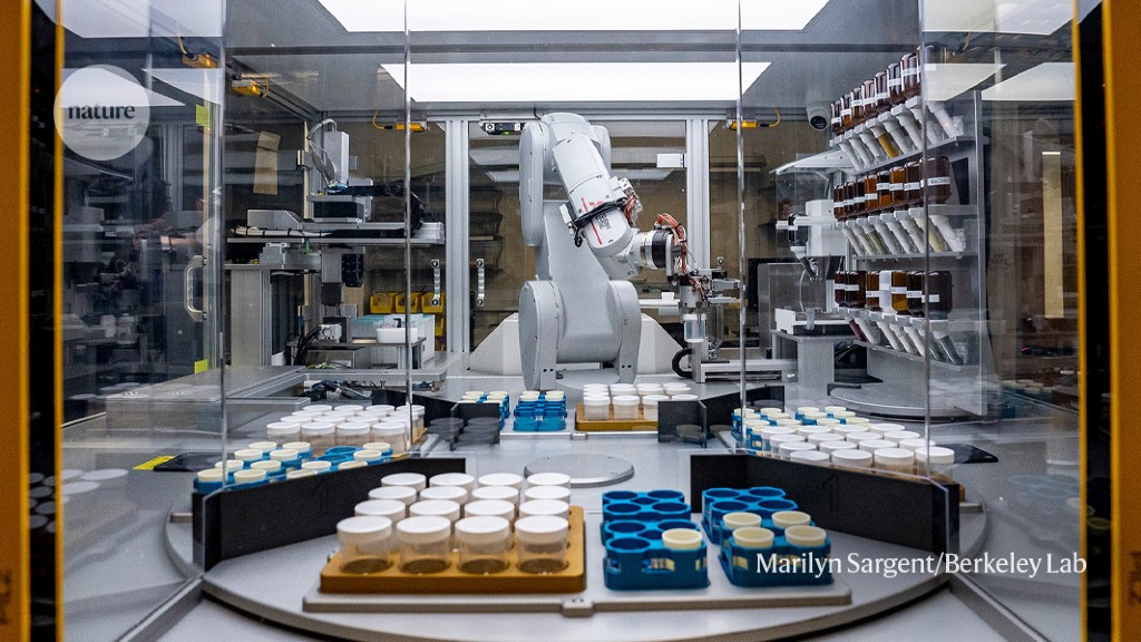
Predicting the existence of a material is one thing, but making it in the lab is quite another. That is where the A-Lab comes in. Gerbrand Ceder, a materials scientist from the University of California, Berkeley, and the lead of the A-Lab team, said that they now have the capability to rapidly make these new materials.
Still, it’s clear that systems such as GNoME can make many more computational predictions than even an autonomous lab can keep up with, says Andy Cooper, academic director of the Materials Innovation Factory at the University of Liverpool, UK. “What we really need is computation that tells us what to make,” Cooper says. For that, AI systems will have to accurately calculate a lot more of the predicted materials’ chemical and physical properties.
The synthesis of hundreds of thousands of compounds is the result of centuries of laboratory work and is not related to the development of organic chemistry. Yet studies suggest that billions of relatively simple inorganic materials are still waiting to be discovered3. So where to start looking?
The A-Lab gave the targets to the machine-learning models for cross-checking after the team identified 58 targets from the Materials Project database.
The A-Lab, housed at LBNL, uses state-of-the-art robotics to mix and heat powdered solid ingredients, and then analyses the product to check whether the procedure worked. The set-up took 18 months to build. The biggest challenge was to make the system truly autonomously, so that it could plan experiments, interpret data and make decisions. The innovation is under the hood, says Ceder, but robots are great fun to watch.
Stable crystal discovery by machine-learning a simple model for oxidation-state balancing in a single crystal structure: applications to Materials Project 16 and OQMD 17
GNoME discoveries aim to extend the catalogues of known stable crystals. The Materials Project 16 and the OQMD 17 are not the only work we have done in this area. snapshots of the two datasets saved at a fixed point in time is what GNo ME-based discoveries use for reproducibility. The data from the Materials Project as of March and the OQMD as of June were used. The catalogue of stable crystals is achieved through the use of these structures as the basis for all discovery. The two groups could get even more crystal discoveries by further updating and incorporating their discoveries.
“Scientific discovery is the next frontier for AI,” says Carla Gomes, co-director of the Cornell University AI for Science Institute in Ithaca, New York, who was not involved in the research. That is what motivates me to find this so exciting.
Structural substitution patterns are based on data-mined probabilities from ref. It was 22. That work introduced a probabilistic model for assessing the likelihood for ionic species substitution within a single crystal structure. The probability of substitution is calculated by using a model that is similar to a feature model. The model is simplified so that it’s 0 or 1 if a specific substitution pair occurs, and there’s a weighting for the likelihood of the substitution. The resulting probabilities have been helpful, for example, in discovering new quaternary ionic compounds with limited computation budgets.
The inputs for evaluation by machine-learning models need to have unique ratios between elements. Enumerating the combinatorial number of reduced formulas was found to be too inefficient, but common strategies to reduce such as oxidation-state balancing was also too restrictive, for example, not allowing for the discovery of Li15Si4. In this paper, we introduce a relaxed constraint on oxidation-state balancing. We begin by analyzing the oxidation states from the Semiconducting Materials byAnalogy and Chemical Theory (SMACT) 57 with 0 for metallic forms. We allow for up to two elements to exist between two ordered oxidation states. The flexibility of composition generation around oxidation-state-balanced ratios is greatly improved by this approach.
The figures show how the model’s generalization abilities scales with training set size. In the next picture. 1e, the training sets are sampled uniformly from the materials from the Materials Project and from our structural pipeline, which only includes elemental and partial substitutions into stable materials in the Materials Project and the OQMD. The training labels are the final formation energy at the end of relaxation. The test set is constructed using 10,000 random compositions from the SMACT. Test labels are the final formation energy at the end of the AIRSS relaxation, for crystals that AIRSS and DFT (both electronically and ionically) converged. The risk of label leaks between the testing set fromAIRSS and the training set from the structural pipeline is minimal because we apply the same composition-based hash filters on our datasets.
As we describe in Supplementary Note 5, not all DFT relaxations converge for the 100 initializations per composition. For certain compositions only a few initializations converge and that’s it. One of the main difficulties arises from not knowing a good initial volume guess for the composition. We try a range of initial volumes ranging from 0.4 to 1.2 times a volume estimated by considering relevant atomic radii, finding that the DFT relaxation fails or does not converge for the whole range for each composition. Prospective analysis did not uncover why most AIRSS initialization fail for certain compositions.
When there are two atoms less than a distance cutoff, the edges are drawn in the graph. Compositional models default to forming edges between all pairs of nodes in the graph. The models update latent node features through stages of message passing, in which neighbour information is collected through normalized sums over edges and representations are updated through shallow MLPs36. After several steps of message passing, a linear readout layer is applied to the global state to compute a prediction of the energy.
Following Roost (representation learning from stoichiometry)58, we find GNNs to be effective at predicting the formation energy of a composition and structure.
A careful balance is needed between making sure the neural networks trained on the dataset are stable and promoting new discoveries. New structures and prototypes are out of the distribution of models, but we hope that the models are still capable of extrapolating and yielding reasonable predictions. This is out-of-distribution detection problem is worsened by the implicit domain shift, which means that models are trained on relaxed structures but evaluated before relaxation. To counteract these effects, we make several adjustments to stabilize test-time predictions.
The test set on which energy predictions are evaluated is created using a random split over different crystal structures. However, as the GNoME dataset contains several crystal structures with the same composition, this metric is less trustworthy over GNoME. The test error does not provide a measurement of how well the model generalizes to new compositions, but having several structures in the same composition reduces test error. The paper has examples to the training and test sets, and a reduced formula for each composition. This ensures that there are no overlapping compositions in the training and test sets. We use a standard MD5 formula, take modulo 100 and threshold at 85, and convert the hexadecimal output to an integer.
Although neural network models offer flexibility that allows them to achieve state-of-the-art performance on a wide range of problems, they may not generalize to data outside the training distribution. Using an ensemble of models is a simple, popular choice for providing predictive uncertainty and improving generalization of machine-learning predictions33. This technique simply requires training n models rather than one. The prediction corresponds to the mean over the outputs of all n models; the uncertainty can be measured by the spread of the n outputs. We use 10 graph networks when training machine-learning models for stability prediction. Moreover, owing to the instability of graph-network predictions, we find the median to be a more reliable predictor of performance and use the interquartile range to bound uncertainty.
Active-Learning Simulations of Structures for DFT Verification, Materials Project, and the pymatgen-based MPNonSCFSet
For active-learning setups, only the structure predicted to have the minimum energy within a composition is used for DFT verification. For an in-depth evaluation of a specific composition family, we use clustering-based reduction strategies. In particular, we take the top 100 structures for any given composition and perform pairwise comparisons with pymatgen’s built-in structure matcher. The minimum energy structure is used as a cluster representation on the graph of pairwise similarities. This provides a scalable strategy to discovering polymorphs when applicable.
The VASP is used in DFT calculations with the PBE41 and PAW40,60 potentials. The Materials Project workflows are reflected in our DFT settings. We use consistent settings with the Materials Project workflow, including the Hubbard U parameter applied to a subset of transition metals in DFT+U, 520 eV plane-wave-basis cutoff, magnetization settings and the choice of PBE pseudopotentials, except for Li, Na, Mg, Ge and Ga. For Li, Na, Mg, Ge and Ga, we use more recent versions of the respective potentials with the same number of valence electrons. For all structures, we use the standard protocol of two-stage relaxation of all geometric degrees of freedom, followed by a final static calculation, along with the custodian package23 to handle any VASP-related errors that arise and adjust appropriate simulations. For the choice of KPOINTS, we also force gamma-centred kpoint generation for hexagonal cells rather than the more traditional Monkhorst–Pack. We assume ferromagnetic spin initialization with finite magnetic moments, as preliminary attempts to incorporate different spin orderings showed computational costs that were prohibitive to sustain at the scale presented. The AIMD simulations use the NVT ensemble with a 2-fs time step.
For validation purposes (such as the filtration of Li-ion conductors), bandgaps are calculated for most of the stable materials discovered. We automate bandgap jobs in our computation pipelines by first copying all outputs from static calculations and using the pymatgen-based MPNonSCFSet in line mode to compute the bandgap and density of states of all materials. A full analysis of bandgaps is a promising avenue for future work.
r2SCAN is an accurate and numerically efficient functional that has seen increasing adoption from the community for increasing the fidelity of computational DFT calculations. This functional is provided in the upgraded version of VASP6 and, for all corresponding calculations, we use the settings as detailed by MPScanRelaxSet and MPScanStaticSet in pymatgen. The r2SCAN functionals require the use of PBE52 or PBE54 potentials, which are slightly different from the PBE equivalents used elsewhere in the paper. To speed up computation, we perform three jobs for every SCAN-based computation. We precondition with the updated PBE54 potentials by running a relaxation job under the MPRelaxSet settings. This preconditioning step greatly speeds up SCAN computations, which—on average—are five times slower and can otherwise crash on our infrastructure owing to elongated trajectories. Then we relax with the r2SCAN functional, followed by a computation.
To compute decomposition energies and count the total number of stable crystals relative to previous work16,17 in a consistent fashion, we recalculated energies of all stable materials in the Materials Project and the OQMD with identical, updated DFT settings as enabled by pymatgen. Furthermore, to ensure fair comparison and that our discoveries are not affected by optimization failures in these high-throughput recalculations, we use the minimum energy of the Materials Project calculation and our recalculation when both are available.
The method used to count the number of materials is available in the pymatgen.analysis.dimensionality package.
Source: Scaling deep learning for materials discovery
High-throughput identification of Li/Mn transition metal oxide conductors using machine-learning models, with application to Gnome and Apache Beam
The estimated number of viable Li-ion conductors reported in the main part of this paper is derived using the methodology in ref. 46 in a high-throughput fashion. This methodology involves applying filters based on bandgaps and stabilities against the cathode Li-metal anode to identify the most viable Li-ion conductors.
The Li/Mn transition metal oxide family is discussed in the ref. 25 to analyse the capabilities of machine-learning models for use in discovery. In the main text, we compare against the findings in the cited work suggesting limited discovery within this family through previous machine-learning methods.
In Fig. 3a, we present the classification error for predicting the outcome of DFT-based molecular dynamics using GNN molecular dynamics. ‘GNoME: unique structures’ refers to the first step in the relaxation of crystals in the structural pipeline. The first DFT step is relaxation and we are training on the forces on each atom. The different training subsets are created by randomly sampling compositions in the structural pipeline uniformly. ‘GNoME: intermediate structures’ includes all the same compositions as ‘GNoME: unique structures’, but has all steps of DFT relaxation instead of just the first step. The Red diamond refers to the same GNG interatomic potential that was trained on the data from M3GNet which includes three relaxation steps per composition.
For efforts in machine learning, GNoME models make use of JAX and the capabilities to just-in-time compile programs onto devices such as graphics processing units (GPUs) and tensor processing units (TPUs). Graph networks implementations are based on the framework developed in Jraph, which makes use of a fundamental GraphsTuple object (encoding nodes and edges, along with sender and receiver information for message-passing steps). We make some great use of JAX MD for processing crystal structures, along with TensorFlow for parallelized data input64.
The main part of the paper describes an overview of the generation and filter process and how Apache Beam can be used to distribute processing to a large group of workers. For example, billions of proposal structures, even efficiently encoded, requires terabytes of storage that would otherwise fail on single nodes.
Source: Scaling deep learning for materials discovery
NequIT potential 30 with five layers and one-hot encodings embedded into SiLU for the gated equivariant nonlinearities
We use e3nn-jax library to train a NequIT potential30, with five layers, hidden features, and irreducible representations. The inner cutoff of 4.5 is used for the radial cutoff of 5 and embedded interatomic distances rij. We also use SiLU for the gated, equivariant nonlinearities68. We embed the chemical species using a 94-element one-hot encoding and use a self-connection, as proposed in ref. 30. For internal normalization, we divide by 26 after each convolution. The models are trained with a learning rate of 103 and a batches of 32. Given that high-energy structures in the beginning of the trajectory are expected to be more diverse than later, low-energy structures, which are similar to one another and often come with small forces, each batch is made up of 16 structures sampled from the full set of all frames across all relaxations and 16 structures sampled from only the first step of the relaxation only. We found this oversampling of first-step structures to substantially improve performance on downstream tasks. The learning rate was decreased to a new value of 2 × 10⁻⁴ after approximately 23 million steps, to 5 × 10⁻⁵ after a further approximately 11 million steps and then trained for a final 2.43 million steps. Training was performed on four TPU v3 chips.
$${\mathcal{L}}={\lambda }{E}\frac{1}{{N}{{\rm{b}}}}\mathop{\sum }\limits_{b=1}^{b={N}{{\rm{b}}}}{{\mathcal{L}}}{{\rm{Huber}}}\left({\delta }{E},\frac{{\widehat{E}}{{\rm{b}}}}{{N}{{\rm{a}}}},\frac{{E}{{\rm{b}}}}{{N}{{\rm{a}}}}\right)+{\lambda }{F}\frac{1}{{N}{{\rm{b}}}}\mathop{\sum }\limits{b=1}^{b={N}{{\rm{b}}}}\mathop{\sum }\limits{a=1}^{b={N}{{\rm{a}}}}{{\mathcal{L}}}{{\rm{Huber}}}\left({\delta }{F},-\frac{\partial \widehat{{E}{{\rm{b}}}}}{\partial {r}{{\rm{b}},{\rm{a}},\alpha }},{F}{b,a,\alpha }\right)$$
The structure was trained using the Adam optimizer, which had a learning rate of 2 103 and a size of 16 for a total of 801 epochs. The learning rate dipped to just 2 104 after 601 instances, before we even trained for another 200 instances. We use the same joint loss function as in the GNoME pretraining, again with λE = 1.0, λF = 0.05 and δE = δF = 0.01. The network hyperparameters are the same as the model used in GNoMe pretraining. To enable a comparison with ref. 62, we also subtract a linear compositional fit based on the training energies from the reference energies before training. Training was performed on a set of four V100 GPUs.
Source: Scaling deep learning for materials discovery
Superionic Behaviour at High Temperatures: AIMD and Diffusion Algorithm for the GNoME Database
Following ref. 69, we classify a material as having superionic behaviour if the conductivity σ at the temperature of 1,000 K, as measured by AIMD, satisfies σ1,000K > 101.18 mScm−1. Refer to the original paper for applicable calculations. See Supplementary Information for further details.
The materials for AIMD simulation are chosen on the basis of the following criteria: we select all materials in the GNoME database that are stable, contain one of the conducting species under consideration (Li, Mg, Ca, K, Na) and have a computationally predicted band gap >1 eV. The last criterion is chosen to not include materials with notable electronic conductivity, a desirable criterion in the search for electrolytes. Materials are run in their pristine structure, that is, without vacancies or stuffing. The AIMD simulations were performed using the VASP. The temperature is set at 300 K and set over a span of 5 ps to get to the target temperature. This is followed by a 45-ps simulation equilibration using a Nosé–Hoover thermostat in the NVT ensemble. Simulations are done at a time step.
The first 10 ps of the machine learning molecular dynamics simulation are thrown out for equilibration. From the final 40 ps, we compute the diffusivity using the DiffusionAnalyzer class of pymatgen with the default smoothed=max setting23,70,71.